
Running machine learning on resource-constrained devices is now a reality, thanks to frameworks like TensorFlow Lite Micro (TFLite Micro). TFLite Micro is specifically designed to run machine learning models on microcontrollers and other devices with limited memory, often with only a few kilobytes available. It operates without requiring operating system support, standard C/C++ libraries, or dynamic memory allocation, making it well suited for embedded environments.
The easy way to integrate TensorFlow Lite Micro into your project is by using the ESP-TFLite-Micro component for ESP-IDF. This component features built-in support for ESP-NN, which optimizes neural network functions for faster inference speeds.
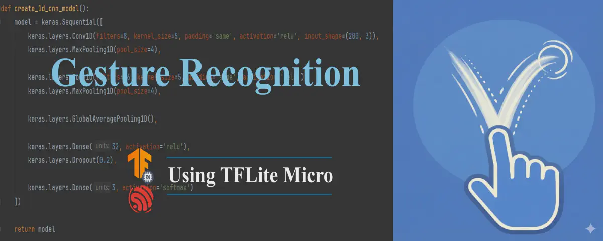
This article guides you through implementing gesture recognition on Espressif SoCs using TFLite Micro. The workflow is organized into four key steps:
- Step 1: Data collection: Gathering gesture data for training.
- Step 2: Model training: Building and training a machine learning model using the collected data.
- Step 3: Model conversion: Converting the trained model into a format compatible with TFLite Micro.
- Step 4: Model deployment: Deploying the model on Espressif SoCs and implementing efficient C++ code for model loading, preprocessing, and inference.
The remainder of the article follows the same step-by-step structure. Background information and practical instructions are grouped under each workflow step to make the end-to-end process easier to follow.
Development Setup#
This workflow uses:
- TensorFlow with Keras API for model deployment.
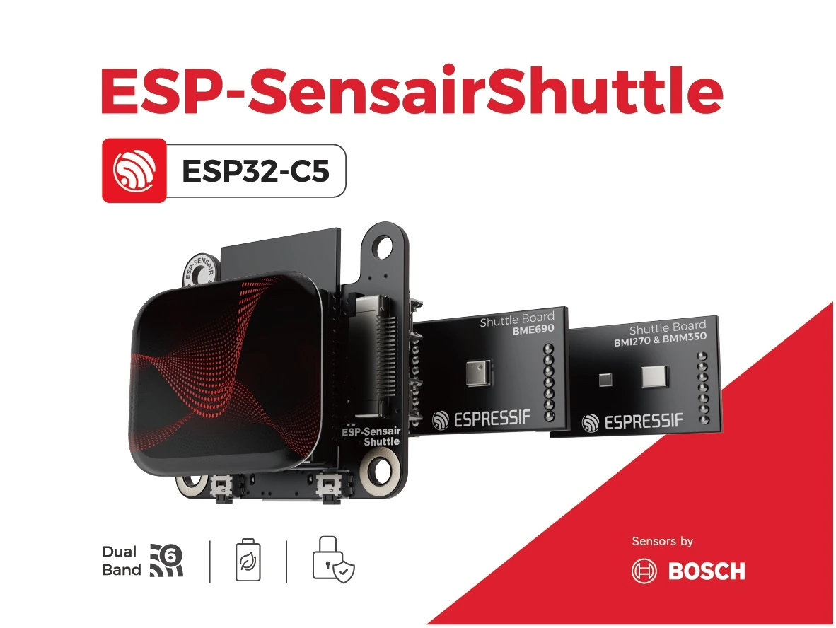
- ESP-SensairShuttle board for data collection and on-device inference.
TensorFlow and Keras#
Model development in this article is based on TensorFlow 2.20.0 with its integrated Keras API. Keras is used for the gesture recognition model development, including model definition, training, evaluation, and export.
If you need a quick refresher on Keras, see the basic classification tutorial on classifying clothing images, which covers model building, compilation, training, evaluation, and prediction.
ESP-SensairShuttle Board#
ESP-SensairShuttle is a development board jointly launched by Espressif and Bosch Sensortec for motion sensing applications and LLM human–machine interaction scenarios, aiming to accelerate the deep integration of multimodal perception and intelligent interaction technologies.
ESP SensairShuttle Introduction
The Factory Demo provides examples for environment sensing, gesture detection, and a compass, making it a convenient reference for becoming familiar with the board before moving on to the gesture recognition workflow.
Step 1: Data Collection#
IMU Data Collection#
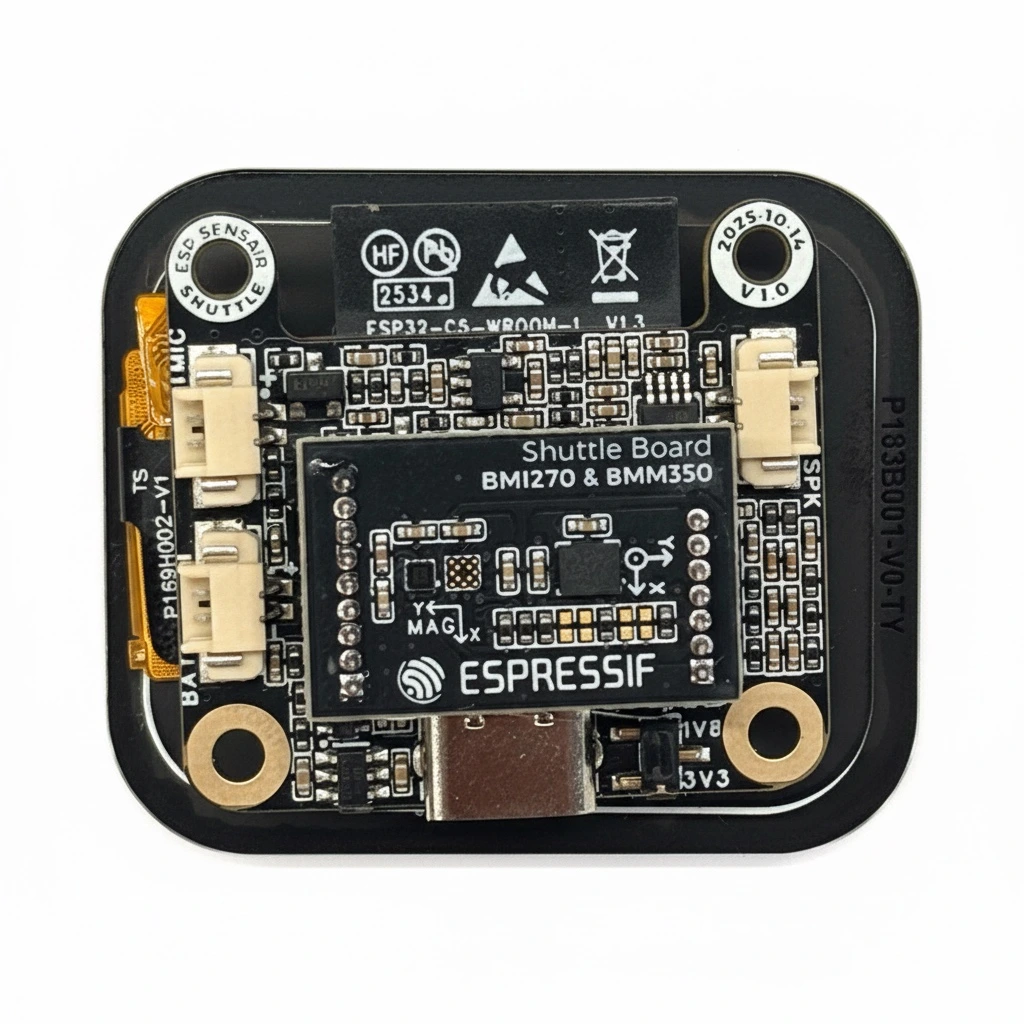
IMU data is collected using the ESP-SensairShuttle Development Board, which features a BMI270 IMU sensor. When a specific gesture is performed, the three-axis angular velocity changes. Gesture recognition is achieved by detecting these changes in angular velocity. The workflow presented here can also serve as a reference for data collection and training with other IMU sensors.
ESP SensairShuttle Development Board
BMI270_Sensor is a component used to drive the BMI270 IMU, facilitating the collection of 3-axis angular velocity data.
To collect high-quality data, both manual triggering and threshold triggering are applied. The system enters a “wait for collection” state via a button press, and the sum of the absolute values of the 3-axis angular velocity is used to determine whether to start recording. Finally, the collected data is sent to the PC via serial port. Additionally, specific separator strings are added before and after the serial transmission to facilitate subsequent data parsing.
In this article, three types of gestures are collected: counterclockwise circles, V-shapes, and unknown gestures. The unknown gestures consist of random movements in an idle state, primarily used to distinguish the first two categories. The time-series data is composed of gyr_x1, gyr_y1, gyr_z1, ..., gyr_x200, gyr_y200, gyr_z200, totaling 600 data points.
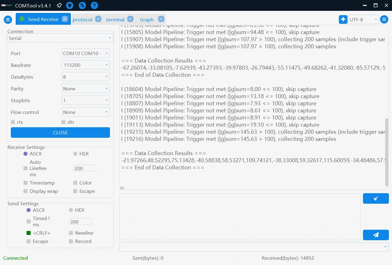
Data Collection
Counterclockwise Gesture
V-shape Gesture
Data Preprocessing#
The gesture data collected over the serial port is first stored in .txt files, and then organized into .csv files using a script. The dataset used in this article can be downloaded here.
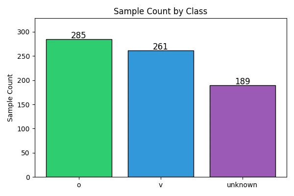
Data Distribution
The preprocessing script reads the collected .csv files, assigns labels to each gesture category, reshapes every sample into a 200 x 3 tensor, and then splits the dataset into training and test sets using train_test_split. The complete preprocessing and training script is provided later in this article.
Step 2: Model Training#
Model Design#
A lightweight Convolutional Neural Network (CNN) model is designed for gesture recognition. The model employs two 1D convolutional layers for feature extraction, each followed by a ReLU activation function and a max pooling layer to reduce feature map dimensions. A Global Average Pooling layer is then used to reduce the number of parameters. Finally, a fully connected layer maps the features to 3 gesture categories. The specific structure is as follows:
model = keras.Sequential([
    keras.layers.Conv1D(filters=8, kernel_size=5, padding='same', activation='relu', input_shape=(200, 3)),
    keras.layers.MaxPooling1D(pool_size=4),

    keras.layers.Conv1D(filters=16, kernel_size=5, padding='same', activation='relu'),
    keras.layers.MaxPooling1D(pool_size=4),

    keras.layers.GlobalAveragePooling1D(),

    keras.layers.Dense(32, activation='relu'),
    keras.layers.Dropout(0.2),

    keras.layers.Dense(3, activation='softmax')
])
It should be noted that the model structure provided here serves only as a reference. In practical applications, different network architectures may be designed according to specific requirements, such as:
- Increasing the feature dimension of input data: For example, using 6-axis IMU data (accelerometer and gyroscope) to provide richer information.
- Trying different activation functions: Such as LeakyReLU, ELU, etc.
- Adding Batch Normalization layers: To accelerate training convergence and improve model stability.
Training and Evaluation in TensorFlow#
During training, the model is compiled with the following configuration:
- Loss Function:
sparse_categorical_crossentropy, suitable for multi-class classification tasks - Optimizer:
adamoptimizer with a learning rate of 0.001
The above parameter configuration is not the only option. In practical applications, you should flexibly adjust hyperparameters such as loss function, optimizer, and learning rate according to specific task requirements to find the most suitable configuration for the current scenario, thereby achieving better model performance.
The prepared dataset is then used to train the model for 300 epochs with a batch size of 64. The complete script, including data extraction, model creation, training, curve plotting, and model export, is shown below.
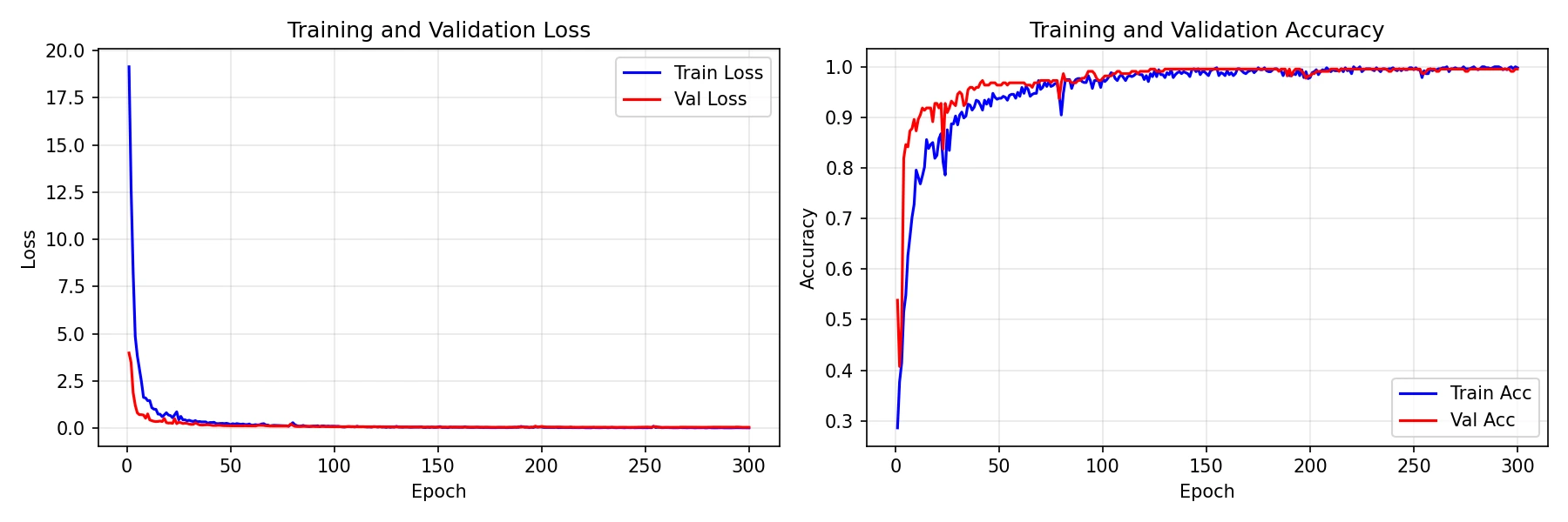
Training Curves
As indicated by the training curves, the model’s accuracy on the test set ultimately stabilizes at 97%. The trained model is then converted to TensorFlow Lite format and deployed to the SensairShuttle.
The complete code for data extraction, model training, and export is as follows:
import matplotlib.pyplot as plt
import numpy as np
import pandas as pd
from sklearn.model_selection import train_test_split
from tensorflow import keras


def extract_data():
    # Read data files
    o_data = pd.read_csv('./o.csv', sep=',', header=None)
    v_data = pd.read_csv('./v.csv', sep=',', header=None)
    unknown_data = pd.read_csv('./unknown.csv', sep=',', header=None)

    # Create labels
    o_label = np.zeros(o_data.shape[0], dtype=int)
    v_label = np.ones(v_data.shape[0], dtype=int)
    unknown_label = np.full(unknown_data.shape[0], 2, dtype=int)

    # Combine feature data and labels (use .values for all to ensure numpy arrays)
    X_raw = np.vstack([o_data.values, v_data.values, unknown_data.values])
    y = np.concatenate([o_label, v_label, unknown_label])

    # Display the number of samples for each class
    print(f"o samples: {o_label.shape[0]}")
    print(f"v samples: {v_label.shape[0]}")
    print(f"unknown samples: {unknown_label.shape[0]}")

    print(f"Total samples: {len(y)}")

    num_samples = X_raw.shape[0]
    num_timesteps = 200  # 200 timesteps
    num_axes = 3  # x, y, z three axes

    # Reshape data: reshape 600 data points in each row into 200x3 matrix
    X = X_raw.reshape(num_samples, num_timesteps, num_axes)

    return X, y


def create_1d_cnn_model():
    model = keras.Sequential([
        keras.layers.Conv1D(filters=8, kernel_size=5, padding='same', activation='relu', input_shape=(200, 3)),
        keras.layers.MaxPooling1D(pool_size=4),

        keras.layers.Conv1D(filters=16, kernel_size=5, padding='same', activation='relu'),
        keras.layers.MaxPooling1D(pool_size=4),

        keras.layers.GlobalAveragePooling1D(),

        keras.layers.Dense(32, activation='relu'),
        keras.layers.Dropout(0.2),

        keras.layers.Dense(3, activation='softmax')
    ])

    return model


def train_model(model, X_train, y_train, X_test, y_test, epochs=30):
    """
    Train the model using Keras fit method
    """
    # Compile the model
    model.compile(
        optimizer=keras.optimizers.Adam(learning_rate=0.001),
        loss='sparse_categorical_crossentropy',
        metrics=['accuracy']
    )

    # Print model summary
    print("Model Summary:")
    model.summary()

    # Train the model
    history = model.fit(
        X_train, y_train,
        validation_data=(X_test, y_test),
        epochs=epochs,
        batch_size=64,
        verbose=1,
        shuffle=True
    )

    return history


def plot_training_curves(history, save_path="training_curves.png"):
    """
    Plot training loss and accuracy curves (train + validation)
    """
    fig, axes = plt.subplots(1, 2, figsize=(12, 4))

    epochs = range(1, len(history.history['loss']) + 1)

    # Loss
    axes[0].plot(epochs, history.history['loss'], 'b-', label='Train Loss')
    axes[0].plot(epochs, history.history['val_loss'], 'r-', label='Val Loss')
    axes[0].set_xlabel('Epoch')
    axes[0].set_ylabel('Loss')
    axes[0].set_title('Training and Validation Loss')
    axes[0].legend()
    axes[0].grid(True, alpha=0.3)

    # Accuracy
    axes[1].plot(epochs, history.history['accuracy'], 'b-', label='Train Acc')
    axes[1].plot(epochs, history.history['val_accuracy'], 'r-', label='Val Acc')
    axes[1].set_xlabel('Epoch')
    axes[1].set_ylabel('Accuracy')
    axes[1].set_title('Training and Validation Accuracy')
    axes[1].legend()
    axes[1].grid(True, alpha=0.3)

    plt.tight_layout()
    plt.savefig(save_path, dpi=150)
    print(f"\nTraining curves saved to {save_path}")
    plt.show()


def save_model_h5(model, filepath):
    """
    Save the model in H5 format
    """
    model.save(filepath)
    print(f"Model saved to {filepath}")


if __name__ == "__main__":
    print("\n=== Data Extraction Phase ===")
    X, y = extract_data()
    X = np.array(X, dtype=np.float32)
    y = np.array(y, dtype=np.int32)
    X_train, X_test, y_train, y_test = train_test_split(X, y, test_size=0.3, random_state=42)
    print(f"Training set: {X_train.shape[0]} samples, Test set: {X_test.shape[0]} samples")

    print("\n=== Model Creation ===")
    model = create_1d_cnn_model()

    print("\n=== Starting Training ===")
    history = train_model(model, X_train, y_train, X_test, y_test, epochs=300)

    print("\n=== Saving Model ===")
    save_model_h5(model, "simple_1dcnn_model.h5")
    print("Training completed!")
Step 3: Model Conversion#
To deploy the trained H5 model on the ESP-SensairShuttle, it first needs to be converted to TensorFlow Lite format so that it can be used by TensorFlow Lite Micro on the target device. In this article, the model is kept in float32 format rather than using integer quantization:
import tensorflow as tf
from tensorflow import keras

model = keras.models.load_model("./model.h5")
converter = tf.lite.TFLiteConverter.from_keras_model(model)

converter.optimizations = [tf.lite.Optimize.DEFAULT]
converter.target_spec.supported_types = [tf.float32]
converter.inference_input_type = tf.float32
converter.inference_output_type = tf.float32

tflite_model = converter.convert()

with open("./model.tflite", "wb") as f:
    f.write(tflite_model)
Full integer quantization can also be explored as a further optimization option to reduce the model size.
Furthermore, to facilitate model loading on the embedded device, the model must be converted into a C/C++ array file:
xxd -i model.tflite > model.cpp
Step 4: Model Deployment#
To implement model inference on the edge, the ESP-TFLite-Micro component must be added to the project, and the model array file imported:
main
├── app_bmi270.cpp
├── app_btn.cpp
├── app_model.cpp
├── app_model_pipeline.cpp
├── CMakeLists.txt
├── idf_component.yml
├── include
│   ├── app_bmi270.h
│   ├── app_btn.h
│   ├── app_model.h
│   ├── app_model_pipeline.h
│   └── model.h
├── Kconfig.projbuild
├── model.cpp
└── motion_estimation.cpp
Here, model.h/model.cpp are the model array files. The ESP-TFLite-Micro component is imported in idf_component.yml:
dependencies:
  idf:
    version: '>=5.5'
  espressif/esp-tflite-micro: 1.3.4
  espressif/bmi270_sensor: 0.1.1
  espressif/button: 4.1.5
In app_model.cpp, a dedicated memory area must be pre-allocated for model inference. The size of this area varies depending on the model and should be adjusted based on actual testing. Furthermore, all operators required by the model need to be registered.
/*
 * SPDX-FileCopyrightText: 2026 Espressif Systems (Shanghai) CO LTD
 *
 * SPDX-License-Identifier: CC0-1.0
 */
#include <string.h>
#include "tensorflow/lite/micro/micro_mutable_op_resolver.h"
#include "tensorflow/lite/micro/micro_interpreter.h"
#include "tensorflow/lite/micro/system_setup.h"
#include "tensorflow/lite/schema/schema_generated.h"
#include "esp_log.h"
#include "freertos/FreeRTOS.h"
#include "freertos/task.h"
#include "freertos/semphr.h"
#include "model.h"
#include "app_model.h"

static const char *TAG = "APP_MODEL";
static const char* kLabels[] = { "Counterclockwise circle", "V", "Unknown" };

// TensorFlow Lite model related
constexpr int kTensorArenaSize = 50000;
uint8_t tensor_arena[kTensorArenaSize];
tflite::MicroInterpreter *interpreter = nullptr;
TfLiteTensor *input = nullptr;
TfLiteTensor *output = nullptr;

void app_model_init()
{
    const tflite::Model *model = tflite::GetModel(model_tflite);
    if (model->version() != TFLITE_SCHEMA_VERSION) {
        MicroPrintf("Model provided is schema version %d not equal to supported "
                    "version %d.",
                    model->version(), TFLITE_SCHEMA_VERSION);
        return;
    }

    static tflite::MicroMutableOpResolver<8> resolver;

    if (resolver.AddSoftmax() != kTfLiteOk) {
        MicroPrintf("Failed to add softmax operator.");
        return;
    }

    if (resolver.AddFullyConnected() != kTfLiteOk) {
        MicroPrintf("Failed to add fully connected operator.");
        return;
    }

    if (resolver.AddMaxPool2D() != kTfLiteOk) {
        MicroPrintf("Failed to add max pool 2D operator.");
        return;
    }

    if (resolver.AddConv2D() != kTfLiteOk) {
        MicroPrintf("Failed to add conv 2D operator.");
        return;
    }

    if (resolver.AddAveragePool2D() != kTfLiteOk) {
        MicroPrintf("Failed to add average pool 2D operator.");
        return;
    }

    if (resolver.AddExpandDims() != kTfLiteOk) {
        MicroPrintf("Failed to add expand dims operator.");
        return;
    }

    if (resolver.AddReshape() != kTfLiteOk) {
        MicroPrintf("Failed to add reshape operator.");
        return;
    }

    if (resolver.AddMean() != kTfLiteOk) {
        MicroPrintf("Failed to add mean operator.");
        return;
    }

    // Create interpreter
    static tflite::MicroInterpreter static_interpreter(model, resolver, tensor_arena, kTensorArenaSize);
    interpreter = &static_interpreter;

    // Allocate memory for model tensor
    TfLiteStatus allocate_status = interpreter->AllocateTensors();
    if (allocate_status != kTfLiteOk) {
        MicroPrintf("AllocateTensors() failed");
        return;
    }

    input = interpreter->input(0);
    output = interpreter->output(0);
}

bool app_model_predict(float (*imu_data)[3], size_t num_samples, app_model_result_t *result)
{
    if (interpreter == nullptr || input == nullptr || output == nullptr) {
        ESP_LOGE(TAG, "Model not initialized");
        return false;
    }

    // Copy IMU data to input tensor
    memcpy(input->data.f, imu_data, num_samples * 3 * sizeof(float));

    // Run inference
    TfLiteStatus invoke_status = interpreter->Invoke();
    if (invoke_status != kTfLiteOk) {
        ESP_LOGE(TAG, "Invoke failed");
        return false;
    }

    // Get output tensor
    float *output_data = output->data.f;
    int num_classes = output->dims->data[1];

    // Find class with maximum probability
    int pred_idx = 0;
    float max_prob = output_data[0];
    for (int i = 1; i < num_classes; i++) {
        if (output_data[i] > max_prob) {
            max_prob = output_data[i];
            pred_idx = i;
        }
    }

    // Store result if requested
    if (result != nullptr) {
        result->class_id = pred_idx;
        result->confidence = max_prob * 100.0f;
        result->class_name = kLabels[pred_idx];
    } else {
        /* Only print if result is not requested (manual mode) */
        printf("Predicted class: %s, confidence: %.1f%%\n", kLabels[pred_idx], max_prob * 100.0f);
        fflush(stdout);
    }

    return true;
}
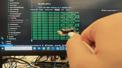
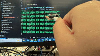
The complete project code is available at gesture_recognition. Please note that this example defaults to automatic inference mode (a long press of the Boot button switches to collection mode, where each press of the Boot button triggers a single data collection). When the sum of the absolute values of the 3-axis angular velocity exceeds the configured threshold, inference is automatically executed, and the category with the highest score within the window is selected as the recognition result.
Conclusion#
This article demonstrated the implementation of a gesture recognition system using TFLite Micro, detailing the complete workflow from data collection and model training to deployment on ESP32 series chips.
The complete project, including Python scripts for data processing, model training, and quantization, along with the C++ inference code and pre-trained models, is available in the esp-sensairshuttle repository.
Feel free to try these examples, implement your own applications, and share your experience!